Using seasonality to identify current and trending requests for promotion

In recent years, SEO has changed a lot in terms of the approach to work, the options for purchasing links have changed, and some have abandoned them altogether. Approaches to query selection have changed, and many automated services have appeared to collect the most complete list of semantics for a website.

Almost all agencies and independent specialists offer and collect large semantics, and there is benefit in this. More requests mean more chances to bring some to the TOP and thereby give results to the client – why he applied.

How is big semantics put together? In short – expanding the structure, collecting queries, parsing hints, clearing semantics from garbage and unnecessary queries. As a result, we get a kernel with targeted queries, if not for one “BUT”! When collecting semantics, no one will take into account the seasonality and trendiness of queries separately; seasonality can be taken into account in general, but not individually, because this takes a lot of time.

In this article I will offer one of the options (I am sure that many of you have your own options and methods), I repeat, this is just one of the options that will help in identifying useful and unnecessary queries in terms of seasonality, trend and demand.

First, you need to put the collected semantics into seasonality measurement in Key Collector, while there are options for measuring by week and by month, we will use measurement by month:

After the measurement, we upload the received data to a file and get a lot of numbers that are difficult to work with, as at first glance, but this is not so.

We will do all calculations in this file; for analysis we will also need the exact frequency of requests and its completeness (Frequency “!” / Frequency), later it will be clear why.

The first stage is the calculation of “rough” dynamics

At this stage, we will try to determine the dynamics of the request for 2 years (it is for this period that seasonal data is uploaded), for this we consider the following:

• The average value for the first year of our unloading (I have it marked in gray);
• Second year average;
• Dynamics on Wed. meanings.

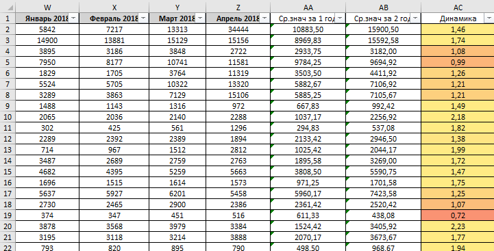
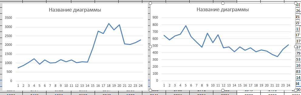
What do we get? And we get an understanding of whether the demand as a whole is growing or not. For example, let’s take a graph for 2 years for a request with dynamics greater than 1. I take a request with dynamics of 2.18:

And now a request with dynamics less than 1, in my case I’ll take a request with dynamics 0.72:

The difference is already noticeable, already at this stage we can say which request is worth using and which one is not interesting to us, because it is losing its demand:

Second phase

At this stage, we calculate the sum of frequencies and dynamics using the obtained figures. I’ll get ahead of myself and say that for many queries “Dynamics on Wed. value” and “Dynamics by amount” will be the same. So, we calculated the sum for the first year, the sum of the frequencies for the second year and the Dynamics:

And yes, the numbers are indeed the same, but why then was it necessary to count it? But why – I sort by “Dynamics of amounts”:

We have identified requests that are just beginning their journey. And they can be very useful in the future.

Third stage

We carry out the first 2 steps, only with the maximum and minimum frequency in each of the years of unloading. As a result, we get the dynamics based on the maximum and minimum points of the graph:

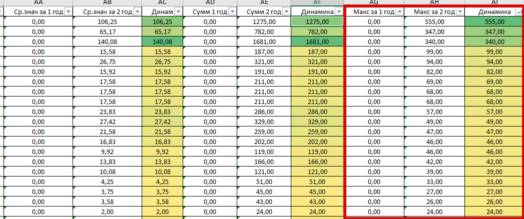
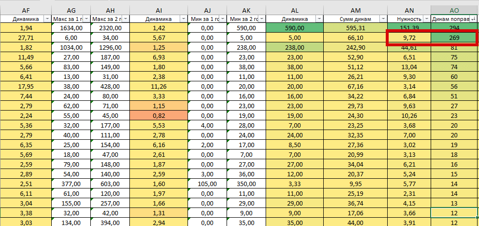
Next, we summarize all the data on the dynamics and get a conditional rating of the request based on seasonality and demand:

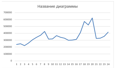
If you look at the graph of queries with the greatest amount of dynamics, we will see something like this – the query is gaining popularity. Most likely, next year it will be even more popular:

But if we look at the graphs of requests with the smallest amount, then we will see dynamics that will not be interesting to any specialist, even if the request is frequent:

Fourth stage

We find queries that will be as “safe” as possible for us, that is, queries that will not have sharp jumps to 0 and will have positive dynamics. Let’s call this value “Need”; it’s easy to calculate – divide the minimum value for year 2 by the maximum for year 2, multiply the resulting value by the sum of the dynamics:

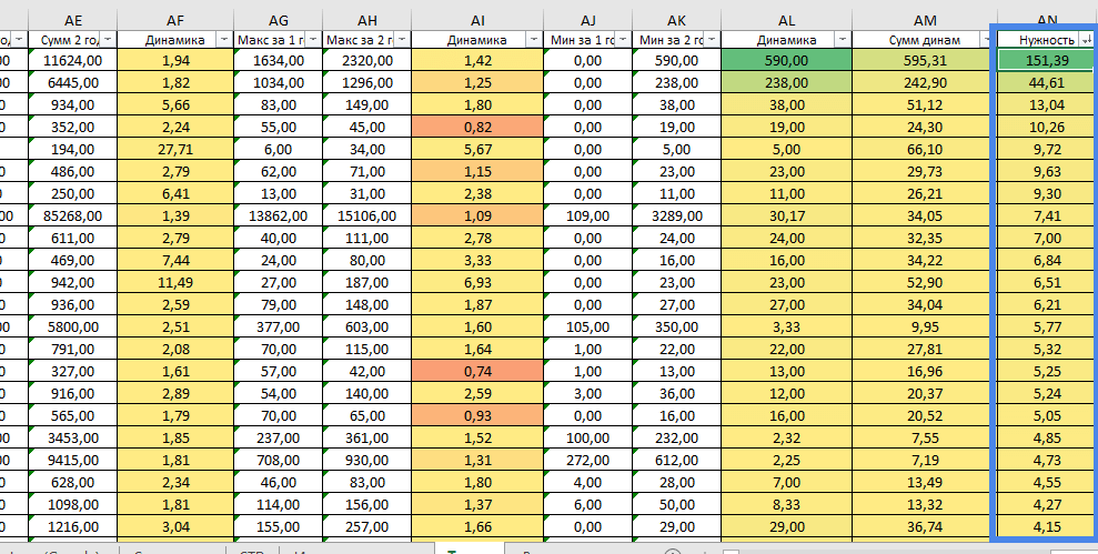
Fifth stage

Since our “Need” does not always work correctly, we need to exclude such cases. To do this, let’s calculate the following value: Multiply the need by the very first dynamics on Wed. values. As a result, we get cases where the request had a very low rating according to “Need”, but in fact it is useful for us. These are the requests that our Corrective Dynamics “pulls up”. Example:

Now let’s look at the query graph. And yes, it is really useful and necessary:

Sixth stage

Let’s clarify our correction dynamics; to do this, we divide the dynamics value by avg. the value of the dynamics of all requests. And then we will display the rating of requests; to do this, we will multiply our final dynamics by the sum of frequencies for 2 years (we are interested in current requests), and we will also multiply all values ​​by 0.00001 so that the numbers are more receptive:

We see a request that is very good, let’s look at its graph, where we will see that this is true:

Seventh stage – final

Here we will need the data that I spoke about earlier, namely:

• Measurement of exact frequency;
• Completeness.

To determine the final rating of a query, you need to multiply the rating obtained in the sixth stage, the exact frequency and completeness:

As a result, we will get very useful queries at the top (if sorted by the resulting rating in descending order) and absolutely unnecessary queries at the bottom. Examples of top query graphs:

And here are the graphs with queries below:

This is what my version of determining the usefulness of queries looks like. At the moment this is just a beta version, and I would like to hear your opinion to help improve this calculation.

Olha Tyshchenko

Editor

Author's page